Background

For many years I have worked New Zealand on the lower shortwave bands, both long and short path. The signal strength is often high even though the forecast program VOACAP indicates that the signal strength should be almost non-existent. The common perception is that the signal is traveling for most of the way in the ionosphere without being attenuated by ground reflections.

Previously, it has been 160 to 40 m, but more recently also 60 m. In favorable circumstances, it has been possible to make SSB contacts when the ZL stations have used 10W. On one such occasion, I have taken an FT-817 and a magnetic loop to try to find the azimuth angle of the incoming wave. I did not get any bearing at all while stations in Europe had sharp dips and a clear bearing. A given conclusion is that the signals from ZL came with a very high angle of incidence. In the past, a low dipole has in some circumstances given much stronger signals than a vertical in ZL and VK.

It would be interesting to have it confirmed by direct measurements.

Measurement system

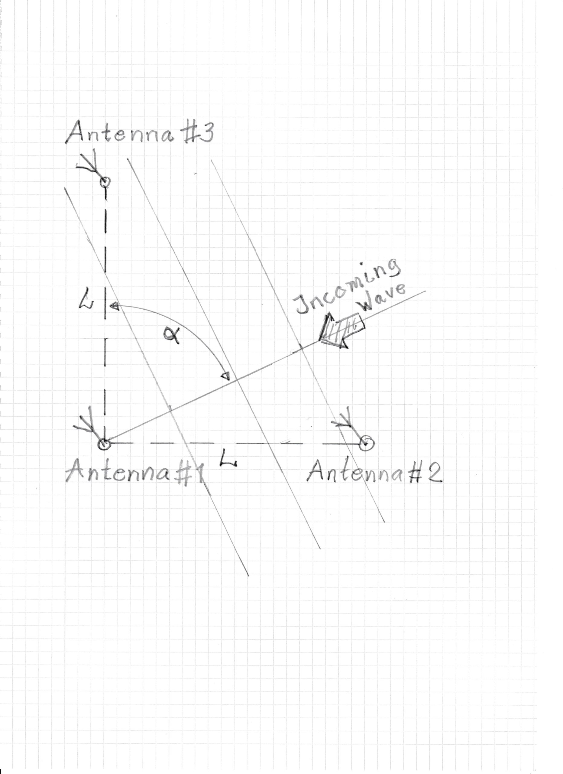
Over the years, many different systems have been studied to measure the angle of incidence. But all have been difficult to realize in practice with limited resources. An appealing solution is a DF system based on the interferometer method. In order to obtain an unambiguous measurement regarding direction, at least three antennas are required, advantageously placed as an L with less than half a wavelength distance. To measure the phase difference between the antennas, a receiver with at least two synchronized channels is required, which is switched between the two legs in the L.

Radio equipment

Recently, Software Defined radios (SDRs) with two phase-locked channels have been available to affordable prices. This makes it possible to measure the phase angle between antennas and build a Direction Finding (DF) system based on the interferometer principle. Such equipment has been available commercially, for example from Rhode & Schwartz, but at a very high price.

An early application is found in SM5BSZ (Leif Åsbrink’s) system for polarization optimization at EME communication. There, his software LINRAD is used together with a two-channel SDR from AFEDRI. For shortwave, there is AFE822x SDR-Net. A shortwave application is described here. Alex at Afedri also has a four-channel SDR, but I have not found any public software that can handle four channels.

The idea was to buy an AFE822x, but after contact with Alex it turned out that it was not possible to get it delivered to my door and I could not visit Postnord’s parcel delivery point due to the Corona pandemic. Instead, I bought an RSP DUO from SDRPlay from Limmared with home delivery. It uses the software SDRUno, which has a function to control and also optimize the phase between the two channels.

The phase control worked as intended by optimizing the signal from two antennas or controlling the phase to minimize a disturbance coming from a direction other than the intended signal. However, the phase relationship between the antennas was completely unpredictable. For tests with a measuring transmitter and two antennas separated by a quarter wavelength, the signals shall have a 90 degree phase difference when the transmitter is along the connection line and a 0 degree difference when it is perpendicular to the connection line. After contacting SDRPlay support, I found out that the channels are synchronized, but at each start of “Diversity mode” a fixed but arbitrary phase difference arises between the channels (Tuner 1 and Tuner 2). While working on this and using fixed delay lines, I discovered that the inputs on the two channels affected each other if they were interconnected. It was therefore important to separate them. I used a simple resistor network.

To compensate for the fixed phase difference between the channels, it is necessary to switch the antennas between the channels.

Assume that ϕ1 is the signal in antenna nr1 and ϕ2 is the signal in antenna nr2.

We are looking for (ϕ2 – ϕ1)

First connect antenna No. 1 to Tuner1 and antenna No. 2 to Tuner2. Let k be the fixed delay.

The phase difference read in SDRuno is ϴ1.

Then connect No. 1 to Tuner2 and antenna No. 2 to Tuner1.

The phase difference read is then ϴ2.

It is illustrated below:

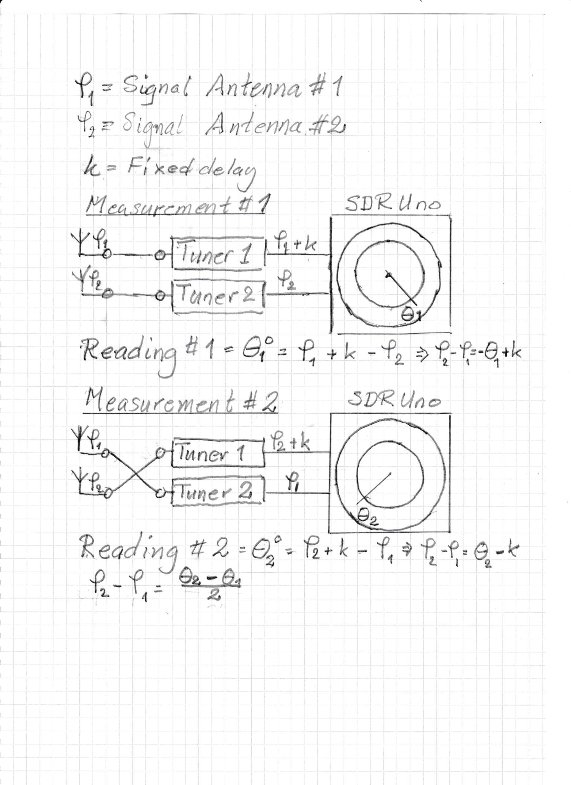
Thus (ϕ2 – ϕ1) = (ϴ2 – ϴ1) / 2

Here one must take into account the condition that the phase difference can never be greater than the electrical distance between the antennas, which may seem to be the case due to the indeterminate constant k.

Example:

ϴ1 = 340° and ϴ2 = 10°. (ϴ2 – ϴ1)/2 is then either 165° or 15°. If the distance between the antenna elements is less than 165 ͦ, eg 90° for λ/4, select 15 °. The phase angles are then ϴ1 = -20° and ϴ2 = 10°.

If (ϕ2 – ϕ1)> 0, the signal comes first to antenna no. 2 and then to antenna no. 1.

If (ϕ2 – ϕ1) <0, the signal comes first to antenna no. 1 and then to antenna no. 2.

If (ϕ2 – ϕ1) = 0, the signal arrives simultaneously at antenna no. 1 antenna no. 2.

A corresponding calculation is made for the other leg in the L and we call (ϕ3 – ϕ1) ϴ3.

That is, and (ϕ3 – ϕ1) = (ϴ3 – ϴ1)/2

Calculation of the angles

 The azimuth angle α is calculated as:

α = arctan((ϕ2 – ϕ1)/(ϕ3 – ϕ1)) degrees

The angle of incidence β is calculated as:

β = arccos(√((ϕ2 – ϕ1)² + (ϕ3 – ϕ1)²)/(L*360/λ)) degrees

Where λ is the wavelength and L is the distance between the antennas.

Practical difficulties

Sensitivity analysis

Small errors in the reading of the measured values give large errors in the result, especially for the angle of incidence β.

A calculation example:

Assume that an incoming wave has an azimuth angle α of 45 degrees and an angle of incidence β of 20 degrees. The distance L between antenna 1 and 2 and antenna 1 and 3 is 90 degrees (eg 10.7 m on 7 MHz).

Then (ϕ2 – ϕ1) = (ϴ2 – ϴ1)/2 and (ϕ3 – ϕ1) = (ϴ3 – ϴ1)/2 must be equal and have the value 59.8 degrees.

Variations in the signal make the reading very difficult.

Assume that (ϴ2 – ϴ1)/2 is measured to 50 degrees. A small error when trying to measure a varying signal.

And that (ϴ3 – ϴ1)/2 is measured to 55 degrees. Also a very small error in the reading.

By inserting these values in the formulas above, α is calculated to 42 degrees. Not so much wrong with the real α, which is 45 degrees. β, on the other hand, is calculated to 34 degrees, which is very different from the actual value of 20 degrees.

The diversity function in SDRuno

It also turns out that the automatic optimization function in SDRUno is only gives a steady reading for very strong and stable signals to find ϴ. For weaker signals the value flutters a lot and it takes measurement series over several minutes with many tens of measured values to get a statistically correct value. Therefore, you must use the Diversity function manually and measure at a minimum, which is sharper than the maximum, and subtract 180 degrees from the measured value. Even so, a certain hysteresis in amplitude poses problems when it comes to finding a sharp minimum in SDRUno.

Topography of the measurement site and soil conditions

My DF antennas are up on a hill with relatively steep sides and an uneven mountainous terrain in the surroundings. The ideal is a flat field with a large extent. How much it affects the measurements has not been determined.

Another thing to consider is ground conductivity. The antennas are only sensitive to the vertical component of the incoming wave. The vertical component of an incoming wave is tilted when it moves along the surface. The tilt is greater the poorer the ground conductivity. It is therefore not possible to measure low radiation angles directly. Maybe you can calibrate the error with a measuring transmitter. In experiments with measuring transmitters on the ground a couple of hundred meters away, however, the measured value shows 0 degrees for measurements of 80m. Larger distances are required. It is not clear how much tilt there is at a space wave, but what I have found are calculations and measurements at a ground wave. In that case, the tilt is in the order of 10° at 5 MHz and poor ground conductivity.

The mentioned tilt is used in Beverage antennas

Conducting objects nearby

20 to 30 meters south of the DF antennas is an antenna mast that is a total of 28 meters high with antennas at the top. It probably affects the measured values to some extent.

The antenna system

First I tried a magnetic loop with a diameter of 1 meter with amplifiers like this one with two transistors. The intention was to have a vertically polarized antenna that covered several amateur bands. An advantage is that it works for both low and high radiation angles. The disadvantage is that two loops are required per antenna location because they are not omnidirectional.

Unfortunately, the Signal / Noise ratio, SNR was too bad. Maybe part was due to cross-modulation.

The next attempt was with tuned loops with a diameter of 2 meters. In that case, you have to change the tuning when changing bands. Now the sensitivity was very good and almost in class with my half-wave dipole that sits 21 meters high. Now it was instead the high Q-value that posed problems. It was practically impossible to get the same phase over time in two antennas.

An active antenna called MiniWhip was now tested. It worked fantastically well at very low frequencies, but on shortwave the SNR was not good enough to be used for very weak signals. By increasing the size of the E-probe (antenna), the signal strength could be increased, but the SNR was not improved. Maybe because of cross modulation. Since it only see the vertical component in the E-field, it is insensitive to signals that come with a high radiation angle, eg local signals of 80m.

Thereafter, tuned quarter-wave verticals were set up for 40, 30 and 20m with common feed. In order not to have problems with different phase between the antennas, a copper pipe was driven into ground which would function as “earthing” and give losses and a low Q-value. It turned out that the conductivity in the ground was too poor at one antenna. Therefore, a sparse radial network was laid out on the ground at all the antennas. It consisted of 2×10, 2×7 and 2×5 meters of wire. The feed resistance is around 80 ohms, ie the ground losses are around 50 ohms and the antennas are very broadband with equal phase over the bands.

The distance between the antennas is 10 m and there is a risk that coupling between the antennas will be too high. But the induced power between antennnas turned out to be well below 1%.

The 40m element was then extended approx. 7 m laterally, as an inverted L. This to increase the signal at 60 and 80m. Then the received signal on 40 was too low. Therefore, a blocking circuit for 40m was mounted at the top of the vertical rod and about 3 meters out on the horizontal part a blocking circuit for 60m. This is to increase the antenna signal on 60 and 80 meters. It turned out then that the DF measurements were weird. Damping resistors were mounted at the bottom of the vertical and in the 60m trap. But it did’nt help. So the design was changed back to a 10m vertical radiator. The signal on 80m and 60m was still large enough to overcome the atmospheric and local noise.

Extended antenna system

Today the 18th of October another antenna element was put in service, antenna number 4 in the DF system. It is placed about 42 meters in 245 degree direction from antenna element 3. It consists of a 10 meter long vertical with five 10 meter long counterweights on the ground and a ground rod. The idea is to get a long leg in a southwesterly direction to be able to measure the vertical radiation angle more accurately for signals coming close from SW or NE. Antenna number 3 today has the lowest interference level and is furthest from the large antenna mast.

Antenna 4 is fed with about 63 meters RG-6 with a velocity factor of 0.66. The other antennas are fed with equally long RG-213 cables of about 40 meters.

To calibrate the difference in cable length, a measurement transmitter was placed about 200 meters away perpendicular to the midpoint of the connection line between antenna 3 and 4. The frequency was 3505 kHz and the phase difference between the channels in RSPduo was measured to 154 degrees which is the difference in electrical length for the feeders of antenna 3 and antenna 4 at 3505 kHz.